Thevenin and Norton Theorems: Statement, Procedure and Worked Examples

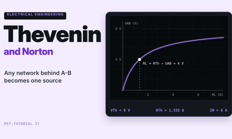
When studying a circuit, we are often interested in only one part of the network: the voltage and current on a load, on the input of an A/D converter, on the lamp connected to a battery. Solving the whole network every time with Kirchhoff’s method (in Italian) is possible but tedious, especially if the load changes value and we want to compare several cases. The Thevenin theorem and its dual, the Norton theorem, solve exactly this problem: everything that sits “behind” two terminals, however complicated, behaves toward the outside like a single source with a single resistance.

In this guide we will look at the statements of the two theorems, their equivalence, a step-by-step procedure for calculating the equivalent voltage, current and resistance (including the open-circuit voltage and short-circuit current method and a note on dependent sources), three worked examples cross-checked with Millman’s theorem (in Italian), maximum power transfer, the extension to alternating current and some practical applications, from the internal resistance of a battery to the output impedance of a voltage divider.

Statement of the Thevenin theorem

Consider a linear network (resistors, ideal voltage and current sources, possibly linear dependent sources) of which we are only interested in two terminals, which we will call A and B. The Thevenin theorem states that:

Any linear network seen from two terminals A and B is equivalent to an ideal voltage source V_Th in series with a resistance R_Th.

• V_Th (Thevenin equivalent voltage) is the voltage U_AB measured across the terminals in open circuit, that is, with the load disconnected.
• R_Th (equivalent resistance) is the resistance seen from terminals A and B when all the independent sources of the network are turned off (or “deactivated”).

The equivalence holds only toward the outside: any load connected between A and B has the same voltage across it and draws the same current both with the original network and with its equivalent. It does not hold, however, for what happens inside the network: the power dissipated in the resistance R_Th, for example, generally does not match the power dissipated in the real resistors. The result was published by Léon Charles Thévenin in 1883, but it had already been derived by Hermann von Helmholtz in 1853; for this reason German-language texts also refer to it as the Helmholtz-Thevenin theorem.

Once V_Th and R_Th are known, the voltage on a load R_L is obtained with a simple voltage divider:

\(U_{AB} = V_{Th}\,\frac{R_L}{R_{Th}+R_L} \qquad I_L = \frac{V_{Th}}{R_{Th}+R_L}\)

Statement of the Norton theorem and equivalence

The Norton theorem is the dual of the previous one. Published almost simultaneously by Edward L. Norton (Bell Laboratories) and by Hans F. Mayer in 1926, it states that:

Any linear network seen from two terminals A and B is equivalent to an ideal current source I_N in parallel with a resistance R_N.

• I_N is the current flowing through terminals A and B when they are short-circuited (I_sc).
• R_N is calculated exactly like R_Th: it is the same resistance, R_N = R_Th.

The two equivalents describe the same network, so they must give the same open-circuit voltage and the same short-circuit current. Imposing these two conditions gives the relations for converting from one model to the other:

\(I_N = \frac{V_{Th}}{R_{Th}} \qquad V_{Th} = I_N\,R_{Th} \qquad R_N = R_{Th}\)

This is the same transformation between a real voltage source and a real current source used to simplify networks one piece at a time. In Millman’s theorem, for example, the E·G term of each branch is precisely the Norton current of that branch: that is why the two topics constantly refer to each other. The choice between Thevenin and Norton is a matter of convenience: Thevenin is more natural when loads are in series, Norton when they are in parallel or when the network already contains current sources.

Step-by-step procedure

Calculating the equivalent always follows the same steps. It is worth keeping them as a checklist:

PROCEDURE FOR THE THEVENIN / NORTON EQUIVALENT
1. Identify terminals A and B and disconnect the load (the part of the network you do NOT want to simplify).
2. Calculate V_Th = U_AB in open circuit, with any method:
   voltage divider, Millman, Kirchhoff, superposition.
3. Calculate R_Th by turning off the INDEPENDENT sources:
   - voltage source  -> replaced by a SHORT CIRCUIT (E = 0)
   - current source  -> replaced by an OPEN CIRCUIT (I = 0)
   then reduce the series and parallel combinations seen from A-B.
4. (As an alternative to step 3) calculate I_sc by shorting A-B
   and derive R_Th = V_Th / I_sc.
5. Draw the equivalent, reconnect the load and calculate U_AB and I_L.
6. Check: at least one result with a second method (Millman or Kirchhoff).

Calculating V_Th in open circuit

With the load disconnected, the current in terminal A is zero, so any resistors in series with the terminal produce no voltage drop. Any technique can be used to calculate U_AB: in simple networks a voltage divider is enough, in two-node networks Millman’s theorem is the fastest, and in networks with several sources the superposition principle is convenient. According to this principle, in a linear network the overall response is the sum of the responses produced by each independent source acting alone (with the others turned off according to the same rules as step 3).

Calculating R_Th with the sources turned off

Turning off a source means setting its imposed quantity to zero: a voltage source with E = 0 imposes a zero potential difference, that is, it behaves as a short circuit; a current source with I = 0 lets no current through, that is, it behaves as an open circuit. The internal resistances of real sources, on the other hand, stay in place. An important consequence: a resistor in series with an ideal current source, once the source is opened, is left floating and does not contribute to R_Th, exactly as it does not appear in the denominator of Millman’s formula.

Open-circuit voltage and short-circuit current method

When series/parallel reduction is awkward, calculate V_Th in open circuit and I_sc with the terminals shorted; their ratio gives the equivalent resistance:

\(R_{Th} = \frac{V_{Th}}{I_{sc}} = \frac{V_{oc}}{I_{sc}}\)

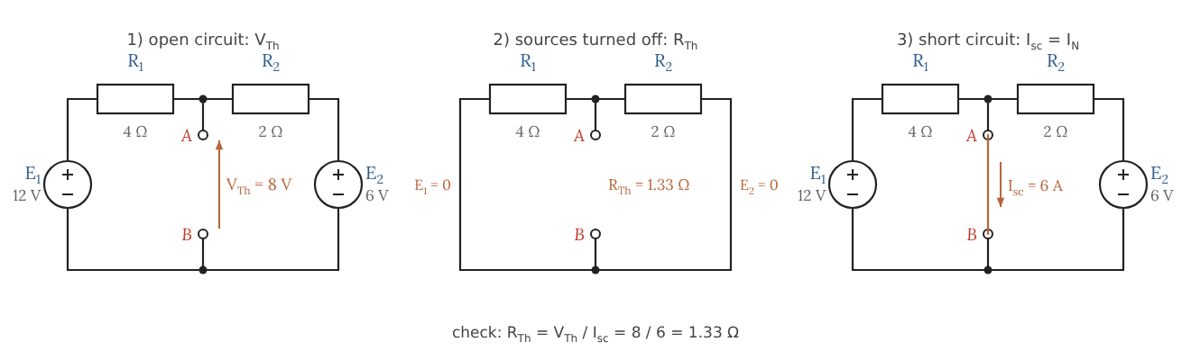
The figure shows the three calculations on the network of example 2: in open circuit we get V_Th, turning off the sources we read R_Th directly, and shorting A and B we get I_sc = I_N. The two paths to R_Th must give the same value, which makes an excellent check.

Networks with dependent sources: the test source

If the network contains dependent sources (controlled by a voltage or current in another branch, as in transistor and amplifier models), these must never be turned off: their value depends on the state of the network. In this case R_Th is found in one of the following two ways:

• with the ratio V_oc/I_sc, if the network also contains independent sources;
• by turning off only the independent sources and applying a test source V_t (or I_t) to the terminals: calculate the current I_t it delivers and set R_Th = V_t/I_t.

In the example in the figure, a dependent current source draws a current k·I_x proportional to the current flowing through R₁. The test source must supply both I_x and k·I_x, so it sees a resistance (1 + k) times smaller than R₁: with R₁ = 1 kΩ and k = 4 we get R_Th = 200 Ω, a value impossible to obtain with series/parallel reductions alone. It is the same mechanism by which feedback lowers the output impedance of an op-amp voltage follower (in Italian).

Example 1: voltage divider with a load

A source E = 12 V feeds a voltage divider made of R₁ = 6 kΩ and R₂ = 3 kΩ; the load R_L is connected in parallel with R₂, between terminals A and B. We want to know how the load voltage changes as R_L varies.

EXAMPLE 1 - data: E = 12 V, R1 = 6 kΩ, R2 = 3 kΩ
V_Th  = E · R2 / (R1 + R2) = 12 · 3 / 9            = 4 V
R_Th  = R1 // R2 = 6 · 3 / (6 + 3)                 = 2 kΩ    (E shorted)
I_N   = V_Th / R_Th = 4 V / 2 kΩ                   = 2 mA    (= E / R1, current in A-B shorted)

Load R_L = 2 kΩ  : U_AB = 4 · 2 / (2 + 2)  = 2.00 V   I_L = 1.00 mA
Load R_L = 10 kΩ : U_AB = 4 · 10 / (2 + 10) = 3.33 V   I_L = 0.33 mA
Load R_L = 1 kΩ  : U_AB = 4 · 1 / (2 + 1)  = 1.33 V   I_L = 1.33 mA

Direct check (R_L = 2 kΩ): R2 // R_L = 1.2 kΩ -> U_AB = 12 · 1.2 / (6 + 1.2) = 2.00 V

The result clearly shows the limit of a voltage divider used as a “power supply”: in open circuit it delivers 4 V, but as soon as the load is comparable to R_Th = 2 kΩ the voltage collapses. The Thevenin equivalent makes this evident with a single number, the output resistance of the divider, and lets you compare several loads without solving the network every time.

Example 2: network with two sources, checked with Millman and Kirchhoff

Two real sources, E₁ = 12 V with R₁ = 4 Ω and E₂ = 6 V with R₂ = 2 Ω, both with the positive pole toward node A, feed in parallel a load R_L = 2 Ω connected between A and B (the circuit of example 2 of the Millman theorem article, without the current source). We calculate the Thevenin equivalent seen by the load and check the result with the other two methods.

Open-circuit voltage by superposition

With the load disconnected, two active branches remain between A and B. We turn on one source at a time, shorting the other:

E1 only (E2 shorted): U' = E1 · R2 / (R1 + R2) = 12 · 2 / 6 = 4 V
E2 only (E1 shorted): U" = E2 · R1 / (R1 + R2) =  6 · 4 / 6 = 4 V
V_Th = U' + U" = 8 V

Check with Millman in open circuit: V_Th = (12/4 + 6/2) / (1/4 + 1/2) = 6 / 0.75 = 8 V

Equivalent resistance and Norton current

R_Th = R1 // R2 = 4 · 2 / (4 + 2) = 1.333 Ω     (E1 and E2 shorted)
I_sc = E1/R1 + E2/R2 = 3 A + 3 A  = 6 A         (A-B shorted)
R_Th = V_Th / I_sc  = 8 / 6       = 1.333 Ω     -> the two methods agree

\(U_{AB} = V_{Th}\,\frac{R_L}{R_{Th}+R_L} = 8\cdot\frac{2}{1.333+2} = 4.8\ V \qquad I_L = \frac{4.8}{2} = 2.4\ A\)

Cross-check

With the load connected, the network has two nodes and three branches: Millman’s theorem gives the voltage between A and B directly.

\(U_{AB}=\frac{12\cdot 0.25 + 6\cdot 0.5}{0.25+0.5+0.5}=\frac{6}{1.25}=4.8\ V\)

With Kirchhoff’s method (one equation at node A and two for the loops, currents I₁ and I₂ entering A from the sources, I_L leaving toward the load) we get:

I1 + I2 = IL
12 - 4·I1 - 2·IL = 0
 6 - 2·I2 - 2·IL = 0
Solution: I1 = 1.8 A   I2 = 0.6 A   IL = 2.4 A   -> U_AB = 2 · 2.4 = 4.8 V

Power balance: sources   12·1.8 + 6·0.6 = 25.2 W
               resistors 4·1.8² + 2·0.6² + 2·2.4² = 12.96 + 0.72 + 11.52 = 25.2 W

The three methods give the same result. Note, however, the difference in “cost”: Kirchhoff and Millman would have to be repeated for every new load value, whereas with the Thevenin equivalent (8 V, 1.333 Ω) a voltage divider is enough. Note also that the power dissipated in R_Th (1.333 · 2.4² = 7.68 W) does not match the power dissipated in R₁ and R₂ (13.68 W): the equivalence holds only toward the load.

Example 3: network with a current source

A current source I_g = 3 mA, with R₄ = 1 kΩ in series, feeds node C; between C and ground there is R₁ = 2 kΩ, from C to terminal A there is R₂ = 2 kΩ, and between A and B there is R₃ = 4 kΩ. We look for the Thevenin equivalent and the voltage on a load R_L = 2 kΩ.

EXAMPLE 3 - data: Ig = 3 mA, R1 = R2 = 2 kΩ, R3 = 4 kΩ, R4 = 1 kΩ
Open circuit: Ig splits between R1 and (R2 + R3)
  U_C  = Ig · [R1 // (R2 + R3)] = 3 mA · (2 · 6 / 8) kΩ = 3 mA · 1.5 kΩ = 4.5 V
  V_Th = U_C · R3 / (R2 + R3)   = 4.5 · 4 / 6                          = 3 V
R_Th (Ig OPEN, so R4 is left floating and does not count):
  R_Th = R3 // (R1 + R2) = 4 // 4                                       = 2 kΩ
Check with I_sc (A-B shorted, R3 shorted out):
  I_sc = Ig · R1 / (R1 + R2) = 3 · 2 / 4 = 1.5 mA  -> R_Th = 3 V / 1.5 mA = 2 kΩ
Norton equivalent: I_N = 1.5 mA in parallel with 2 kΩ
Load R_L = 2 kΩ: U_AB = 3 · 2 / (2 + 2) = 1.5 V   I_L = 0.75 mA   P_L = 1.125 mW

The resistance R₄ in series with the current source appears neither in V_Th nor in R_Th: an ideal current source imposes its current regardless of the resistance in series with it. The result is confirmed by nodal analysis of the complete network (with the load connected we get U_C = 3.75 V and U_AB = 1.5 V). Examples like this also lend themselves to successive source transformations: I_g with R₁ in parallel is equivalent to a 6 V source with 2 kΩ in series; adding R₂ gives 6 V with 4 kΩ, and the divider with R₃ brings us back to 3 V and 2 kΩ.

Maximum power transfer

Once the network has been reduced to V_Th and R_Th, the power on the load is a function of R_L alone:

\(P_L = R_L\,I_L^2 = \frac{V_{Th}^2\,R_L}{(R_{Th}+R_L)^2}\)

The function is zero with the load short-circuited (zero voltage) and tends to zero with the load open (zero current); in between it has a maximum, found by setting the derivative with respect to R_L to zero. The result is the maximum power transfer theorem:

\(R_L = R_{Th} \quad\Rightarrow\quad P_{L,max} = \frac{V_{Th}^2}{4\,R_{Th}}\)

With the data of example 1 (V_Th = 4 V, R_Th = 2 kΩ) the maximum power is 16/8000 = 2 mW and is obtained with R_L = 2 kΩ; in example 3 the 2 kΩ load was already the optimum one (1.125 mW = 3²/(4·2000)). The graph shows the P(R_L) curve, rather flat around the maximum, and the efficiency η = R_L/(R_Th + R_L), referred to the power delivered by the equivalent source alone.

At the maximum point the efficiency is only 50 %: half of the power is lost in R_Th. That is why the matching R_L = R_Th is sought in signal circuits (antennas, transmission lines, audio and RF stages, low-power sensors), where the goal is to extract as much power as possible from a weak source, while in power circuits (the mains grid, batteries, power supplies) we work with R_L much larger than R_Th, to get high efficiency and a stable voltage.

Thevenin and Norton in alternating current

In sinusoidal steady state the two theorems hold unchanged, replacing voltages and currents with phasors and resistances with impedances (Z = R, Z = jωL, Z = 1/(jωC)), as already seen for Kirchhoff (in Italian) and Millman: the equivalent is a voltage source V̄_Th in series with an impedance Z_Th, or a current source Ī_N in parallel with the same impedance. The equivalent is valid at the frequency for which it was calculated.

A short example: a 10 V RMS source at 1 kHz feeds an RC low-pass section (R = 1 kΩ in series, C = 100 nF to ground, the same structure as RC filters); terminals A and B are across the capacitor.

AC EXAMPLE - Vs = 10 V (RMS), f = 1 kHz, R = 1 kΩ, C = 100 nF
Z_C  = 1 / (j·2π·1000·100e-9)          = -j 1591.5 Ω
V_Th = Vs · Z_C / (R + Z_C)            = 8.47 V ∠ -32.1°
Z_Th = R // Z_C = R·Z_C / (R + Z_C)    = (717 - j 450) Ω   (|Z_Th| = 847 Ω ∠ -32.1°)
Resistive load 1 kΩ: |U_AB| = 4.77 V ∠ -17.4°  (also verified by solving the complete network)
Maximum power: Z_L = Z_Th* = (717 + j 450) Ω  -> P_max = |V_Th|² / (4·Re Z_Th) = 25 mW

In AC the maximum power transfer condition becomes conjugate matching: the load impedance must be the complex conjugate of Z_Th, so that the reactances cancel and only the resistive part remains. With a purely resistive load, instead, maximum power is obtained for R_L = |Z_Th| and is lower (about 22.9 mW in the example).

Practical applications: batteries, voltage dividers, output impedance

The battery model

The simplest model of a battery is precisely a Thevenin equivalent: an open-circuit voltage E₀ in series with the internal resistance R_i. Since a short circuit is out of the question, R_i is found by measuring the open-circuit voltage and the voltage under a known load for a short time (the DC load method, used for example by load testers for starter batteries):

CALCULATION EXAMPLE (indicative values, 12 V lead-acid starter battery)
Open-circuit voltage          E0 = 12.7 V
Voltage with a 50 A load      U  = 12.2 V
Ri = (E0 - U) / I = 0.5 V / 50 A = 10 mΩ
Theoretical short-circuit current = 12.7 V / 0.01 Ω = 1270 A   -> never try it!

The model explains why a battery’s voltage drops while the engine is cranking and why an aged battery, with a higher internal resistance, can no longer deliver high currents even though it shows a normal open-circuit voltage. It is a purely ohmic model: it does not describe the capacitive and chemical effects that appear with prolonged or varying loads. For an applied example see the analysis of an automotive battery (in Italian).

Voltage divider feeding a load

Example 1 is the typical situation of a voltage divider that scales down a voltage for an input or a bias point: the open-circuit voltage is E·R₂/(R₁ + R₂), but the source “seen” by the load has a resistance R₁//R₂. The rule of thumb is that the error stays negligible only if the load resistance is much larger than R_Th (with a ratio of 100 the error is about 1 %). The same reasoning applies to a divider with an LDR photoresistor (in Italian) read by a microcontroller: the analog inputs of AVR microcontrollers such as the ATmega328P are optimized for sources with an output resistance of about 10 kΩ or less, so that the internal sampling capacitor charges in time (see Arduino analog inputs (in Italian)). The quantity to compare with that limit is precisely the R_Th of the divider, not the sum of the two resistances.

Output and input impedance

When a datasheet states the “output impedance” of a power supply, of a function generator (typically 50 Ω) or of an amplifier stage, it is giving the R_Th (or Z_Th) of the Thevenin equivalent seen from the output. Symmetrically, the input impedance of the next stage is its load. The ratio between the two determines how much voltage is lost in the connection: to transfer voltage you want a low output impedance and a high input impedance, and this is the role of buffers. Likewise, a multimeter (in Italian) used as a voltmeter is a load (typically on the order of 10 MΩ) connected to the Thevenin equivalent of the point being measured: on high-resistance nodes the reading comes out low.

Common mistakes

COMMON MISTAKES WITH THEVENIN AND NORTON
[ ] Calculating V_Th with the load still connected: V_Th is the OPEN-CIRCUIT voltage.
[ ] Turning off sources the wrong way: voltage -> SHORT CIRCUIT, current -> OPEN.
[ ] Including in R_Th a resistor in series with an ideal current source (it must be excluded).
[ ] Turning off dependent sources: they stay active; use V_oc/I_sc or the test source.
[ ] Getting the polarity of V_Th wrong: the + of the equivalent source goes toward the terminal
    that is at the higher potential in open circuit (if U_AB < 0 the source must be reversed).
[ ] Using the equivalent to calculate powers or currents INSIDE the network: it holds only outside.
[ ] Applying the theorems to nonlinear components (diodes, LEDs, switching transistors)
    without linearizing them: you can simplify the linear part, not the nonlinear component.
[ ] Forgetting that I_N = V_Th / R_Th: the direction of I_N is that of the short-circuit current
    leaving terminal A.
[ ] In AC, using an equivalent calculated at a frequency different from the operating one.
[ ] Measuring I_sc by short-circuiting a real battery or power supply.

Sources and further reading

• MIT OpenCourseWare 6.002, Lecture 3: Superposition, Thévenin and Norton
• D. H. Johnson, "Origins of the Equivalent Circuit Concept: The Current-Source Equivalent", Proceedings of the IEEE, 2003
• Battery University, BU-902: How to Measure Internal Resistance

Related articles

• Passive RC and RL filters: formulas, examples and cutoff frequency
• Non-inverting op-amp configuration
• Inverting op-amp configuration
• Millman's theorem: solving linear networks (in Italian)
• Kirchhoff's method: solving AC and DC linear networks (in Italian)
• Resistors: electrical resistance and resistivity (in Italian)
• Op-amp voltage follower (in Italian)
• Analysis and testing of an automotive battery (in Italian)