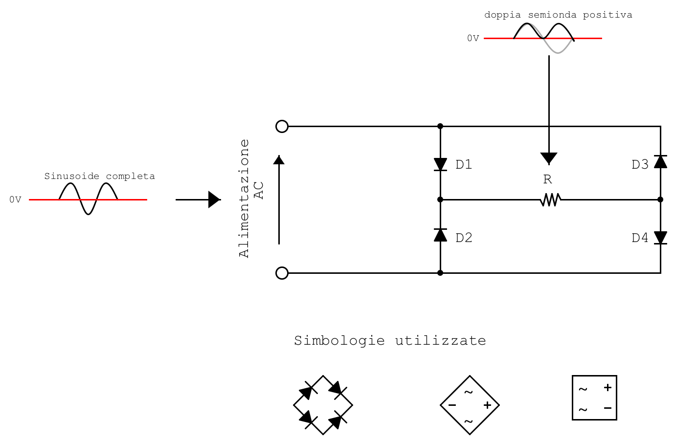
The Graetz bridge rectifier circuit allows an AC voltage to be taken and delivered to the load in the form of positive pulsating waveforms, with a frequency twice that of the supply frequency. This diode system is used in most AC-to-DC power conversion systems.
How the Graetz bridge works
The Graetz bridge may be implemented either as a single integrated component with four terminals or by using four PN-junction diodes. The choice between these two configurations depends on technical requirements such as operating current, insulation, PCB space, and cost factors. When using the integrated version, there are four terminals: two input terminals for the AC supply and two output terminals for the DC supply, marked positive and negative. If we wish to customize the bridge using specific diodes, the following circuit arrangement may be used.
Test circuit and measurements
In our tests, we will use 1N4007 diodes and a 100 kΩ resistor.
On the breadboard, the circuit will be as follows.

We begin our analysis using a multimeter and an oscilloscope. We place the probes across the power supply terminals.
Note: in our case, the supply was provided by a function generator set to Vpp = 10 V and f = 50 Hz.

Since the frequency is 50 Hz, we can determine the period using ( f = 1/T ), obtaining 20 ms. Knowing the peak-to-peak voltage ( V_{pp} ), we can also determine the RMS voltage measurable with the tester set to AC voltage. In this case, our effective voltage is:
\(V_{eff} = \frac{Vpp}{2\cdot \sqrt{2}} = \frac{10}{2\cdot \sqrt{2}} = 3.53V\)Since the supply is alternating and periodic, the average value (dc offset) is zero. Therefore:
\(V_{medio} = 0V\)After completing this preliminary analysis, we observe how the circuit behaves.
Positive half-wave analysis
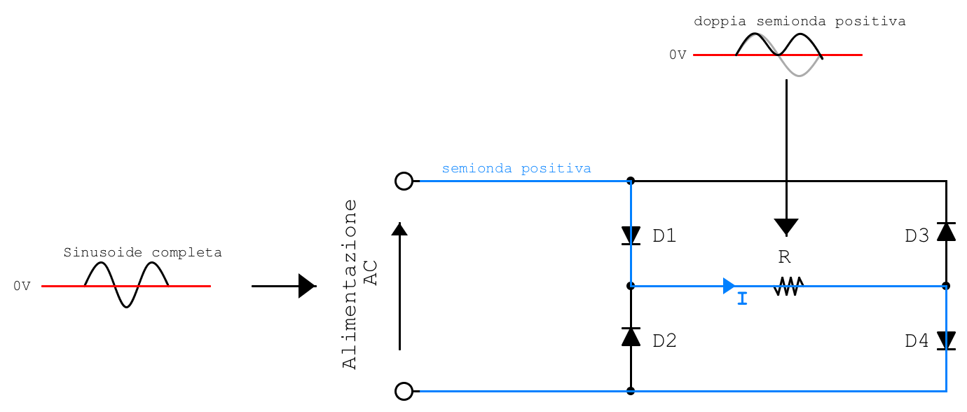
We observe that, since the half-wave is positive, it will flow through the highlighted portion of the circuit, passing through the forward-biased diodes. Naturally, the half-wave must reach a value greater than the threshold voltage of the diodes. The conducting diodes are therefore D1 and D4, and the current flows through the load in the direction indicated by the blue arrow.
 Probe positioned between diode D1 and diode D2 — GND
 We observe that the blue peak voltage ( V_p ) is lower than the yellow ( V_p ). This is due to the voltage drop across the diode.
Negative half-wave analysis
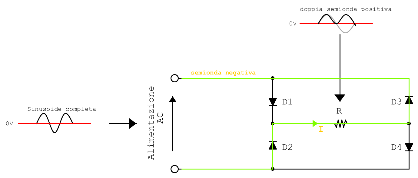
We observe that, since the half-wave is negative, it will flow through the highlighted portion of the circuit, passing through the diodes that are forward-biased for this polarity. The conducting diodes are D3 and D2. Since the half-wave under analysis is negative, the current direction is opposite to that considered in our reference analysis. As a result, the current through the load is restored in the same direction as in the previous example.
Probe positioned between diode D3 and diode D4 — GND
Analysis
We combine the analysis of the positive waveform with that of the negative half-wave. The following graph is obtained.
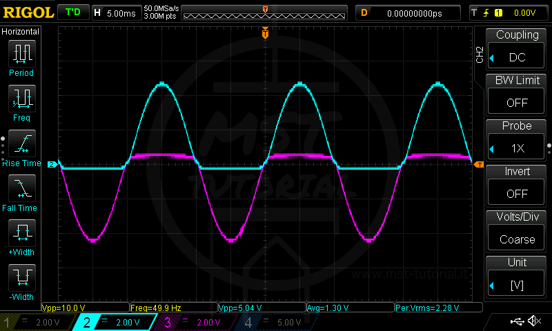
As seen in the previous paragraph, the purple waveform is inverted across the load; therefore, it is appropriate to transform it accordingly.

By superimposing the white signal and the purple signal, we obtain the full-wave rectified waveform.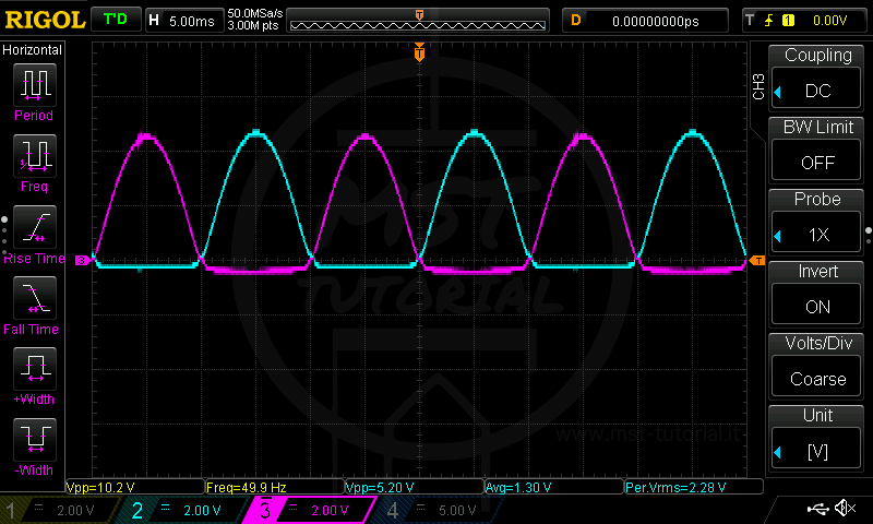
Indeed, by summing the waveforms, we obtain the result shown in blue.

We observe that across the load there is a sequence of positive half-waves, due to the diode-biasing arrangement. Therefore, across the load, a pulsating waveform is obtained at twice the supply frequency, since the period is halved.

As with the single half-wave rectifier, the Graetz bridge also has a short time interval ( t ) during which the load is not supplied. This phenomenon occurs because, during that time interval, the supply voltage is lower than the diode threshold voltage. To overcome this issue, smoothing capacitors can be connected in parallel with the load.
For the rectified and unsmoothed waveform, we can proceed with the mathematical analysis, using the information taken from the penultimate image:
\(V_{eff} = \frac{Vp}{\sqrt{2}} = \frac{5.36}{\sqrt{2}} = 3.79V\)The average value is no longer zero, since the supply is no longer alternating around zero. Therefore:
\(V_{medio} = \frac{2 \cdot Vp}{\pi} = \frac{2 \cdot 5.36}{\pi} = 3.41V\)Note: the measured values reported on this page are being verified. With a 10 Vpp input (Vp,in = 5 V) and two diodes conducting at any time, the peak on the load should be about Vp,out ≈ Vp,in − 2·VF ≈ 3.6–3.8 V rather than 5.36 V; likewise, with a smoothing capacitor the average value should approach the peak and cannot be lower than the unsmoothed average value.
As with the half-wave rectifier, we can calculate the form factor and the ripple factor. The form factor, denoted by ( K_f ), represents the ratio between the RMS value of the voltage and the average value of the signal itself. If the rectification is full-wave, the load is purely resistive, and no smoothing capacitor is applied, we have:
\(K_{f}=\frac{V_{efficace}}{V_{medio}} = \frac{\frac{Vp}{\sqrt{2}}} {\frac{2 \cdot Vp}{{\pi}}} = \frac{\pi}{2\sqrt{2}}= 1.11\)From this value, we can determine the ripple coefficient ( r ), defined as:
\(r=\sqrt{K_{f}^{2}-1} = \sqrt{1.11^{2}-1} = 0.48\)Smoothing
We conclude our introductory analysis of the Graetz bridge by studying its response to smoothing. To smooth the full-wave rectified signal, a capacitor must be connected in parallel with the load in order to exploit its continuous charging and discharging process. Naturally, low-capacitance capacitors will provide poor smoothing.
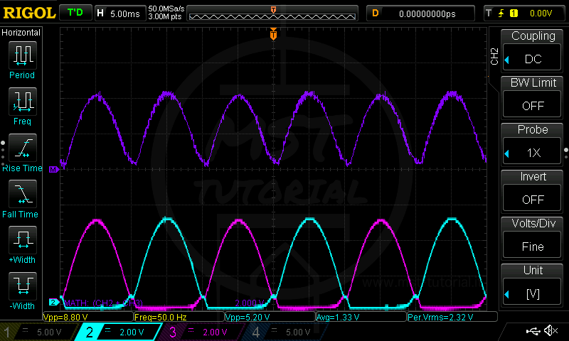 Very poor smoothing: the load is supplied in a pulsating manner, with voltage variations of 5.20 V.
C=100nF R=100K f=50Hz Vmedia=1.72V
 Poor smoothing: the load is supplied in a pulsating manner, with voltage variations of approximately 2 V.
C=1000nF R=100K f=50Hz Vmedia=2.05V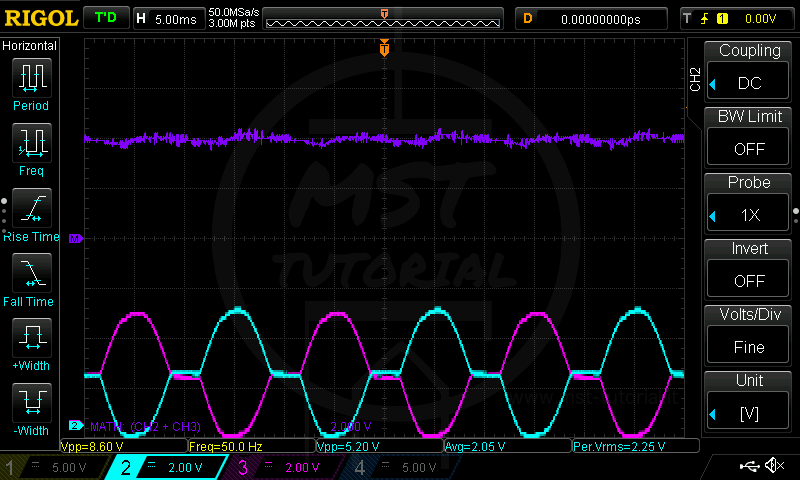 Acceptable smoothing: the load is powered, but with voltage variations of 0.3 V.
 Good smoothing: the load is supplied steadily, with voltage fluctuations below 0.1 V.
Sizing the diodes and the smoothing capacitor
At any time two diodes of the bridge conduct, so the load voltage is reduced by about 2·VF compared with the input peak, while each diode that is not conducting must withstand a peak reverse voltage of about Vp (PIV ≈ Vp). As a first approximation, for a full-wave rectifier the peak-to-peak ripple is ΔV ≈ Iload/(2·f·C), where f is the supply frequency (the ripple frequency is 2f). The capacitor can therefore be sized as:
\(C \approx \frac{I_{load}}{2 \cdot f \cdot \Delta V}\)Related articles